Lab 03: SRV02 Position Control | Anuranan Bharadwaj

Experiment Overview

Position control is fundamental to flight control actuators, robotic arms, gimbal systems, and telescope pointing mechanisms. The challenge is achieving a fast, accurate step response while also tracking continuously-changing reference inputs (like a ramp command) without accumulating position error. This lab designed and implemented a PV controller meeting second-order transient specifications, then demonstrated why adding an integral term is necessary to eliminate the persistent error that appears when the system must track a ramp reference.

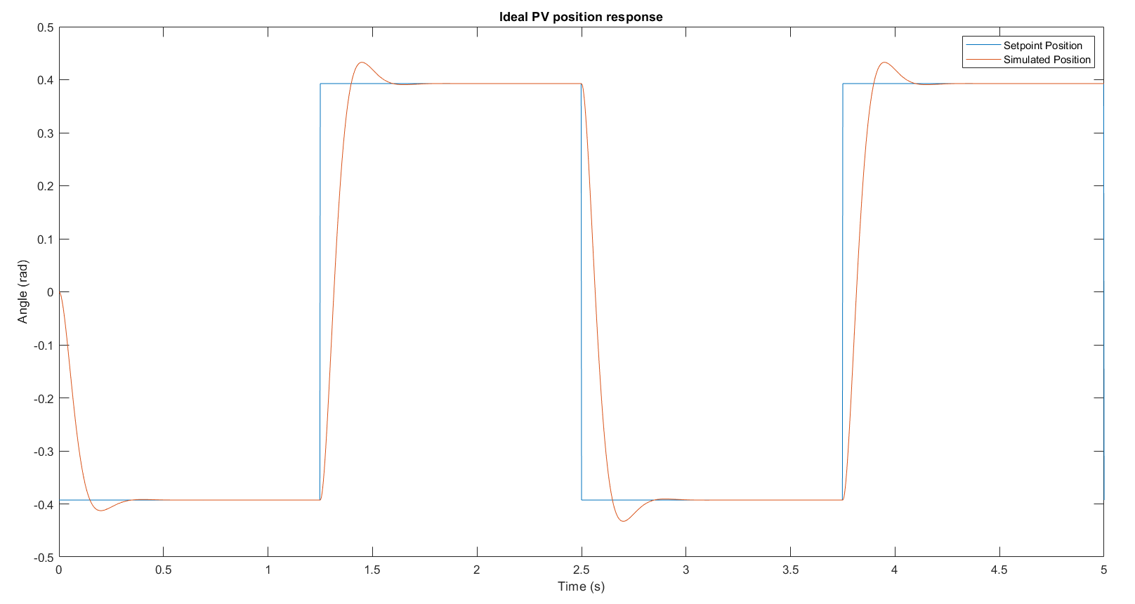
Design PV (proportional-velocity) controller gains from second-order transient specifications: peak time t_p = 0.20 s and percent overshoot PO = 5%
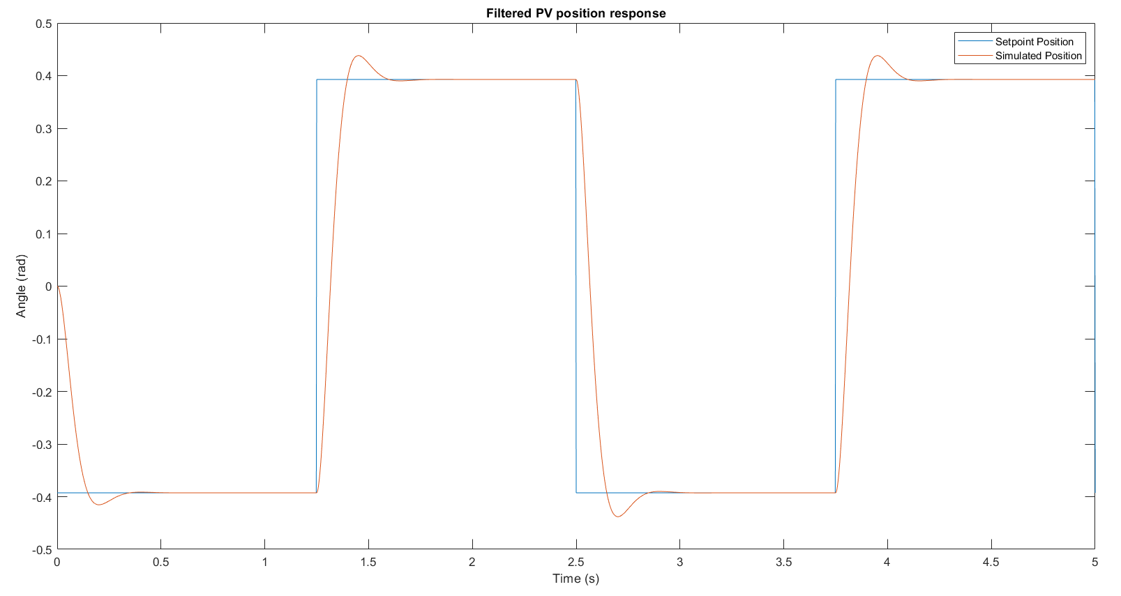
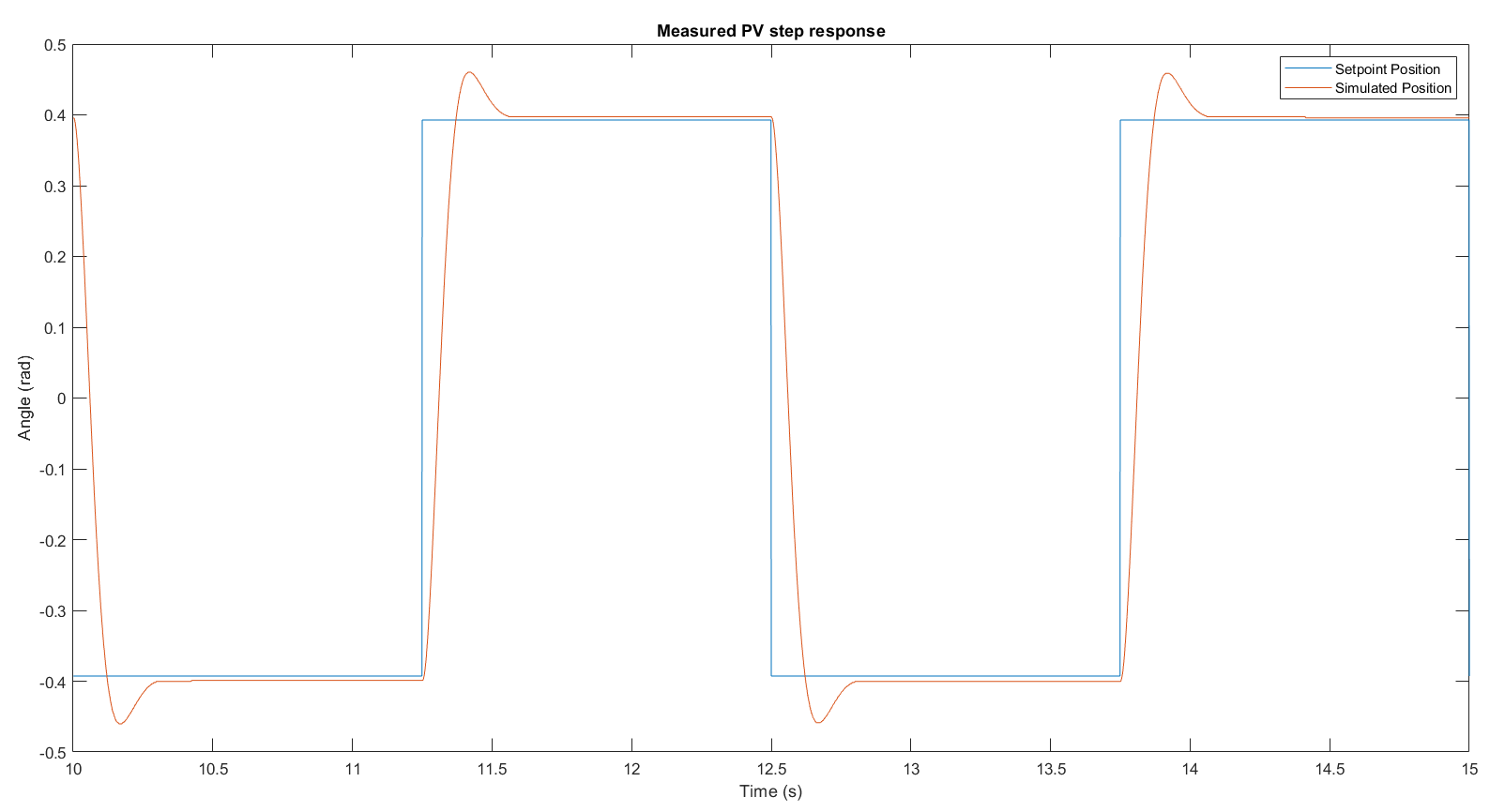
Validate the step response in simulation and on the physical SRV02 hardware
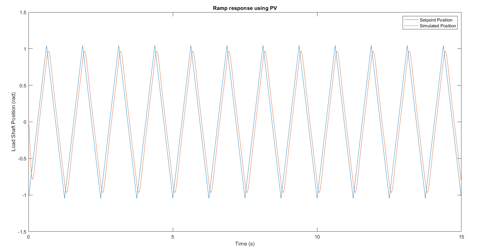
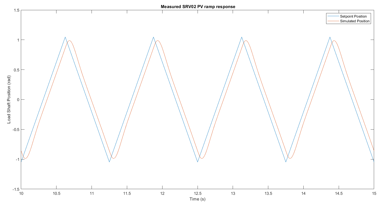
Demonstrate the ramp tracking steady-state error inherent to PV-only control
Add an integral gain to create a PIV controller and reduce ramp steady-state error to near zero

Simulated PV step response – ideal position tracking, t?=0.194 s, PO=5% — Figure 1: Simulated PV step response — t_p=0.194 s, PO=5%

Filtered PV simulated step response showing effect of low-pass filter on velocity feedback — Figure 2: Filtered PV simulated step response — low-pass filter effect on velocity feedback

Implemented PV step response on hardware – t?=0.170 s, PO=7.86%, ess=0.004 rad — Figure 3: Hardware PV step response — t_p=0.170 s, PO=7.86%

Equipment & Tools

Quanser SRV02 rotary servo-motor system
Q2-USB data acquisition board
VoltPAQ power amplifier (V_max = ±10 V)
MATLAB/Simulink with QUARC real-time toolbox
Encoder feedback for position measurement (load shaft optical encoder)

Controller Design

The desired transient specs (t_p = 0.20 s, PO = 5%) were mapped to second-order system parameters: ζ = 0.69 and ω_n = 21.7 rad/s. The PV gains were then derived analytically:

k_p = τω_n² / K = 7.82 V/rad

k_v = (2ζω_nτ − 1) / K = −0.157 V·s/rad

Since a PV controller makes the position loop a Type-1 system, a ramp input produces a predictable non-zero steady-state error e_ss = R(1 + Kk_v) / (Kk_p) = 0.214 rad. Adding an integral gain k_i = 38.9 V/(rad·s) upgraded the controller to PIV, eliminating this error by continuously accumulating and correcting residual position deviation.

PV controller – simulated ramp response, ess=0.213 rad — Figure 4: PV controller — simulated ramp response, e_ss=0.213 rad

PV controller – measured ramp response on hardware, ess=0.186 rad — Figure 5: PV controller — hardware ramp response, e_ss=0.186 rad

PIV controller – simulated ramp response with near-zero steady-state error, ess=0.005 rad — Figure 6: PIV controller — simulated ramp response, e_ss=0.005 rad

Key Results

Test	t_p (s)	PO (%)	e_ss (rad)
Step sim (PV)	0.194	5.0	0
Step impl (PV)	0.170	7.86	0.004
Ramp sim (PV)	—	—	0.213
Ramp impl (PV)	—	—	0.186
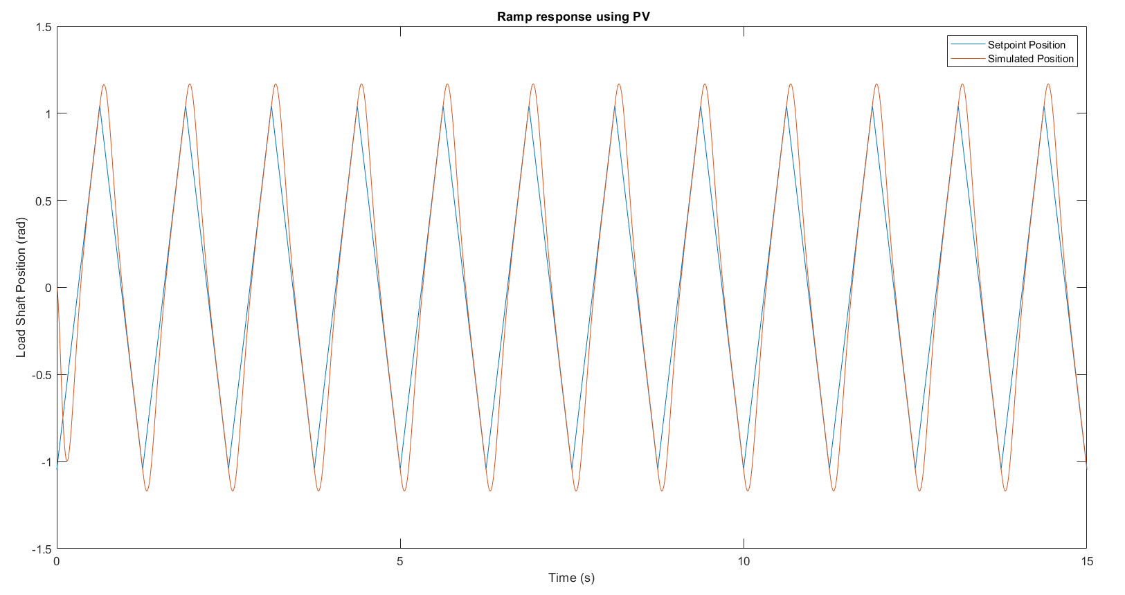
Ramp sim (PIV)	—	—	0.005
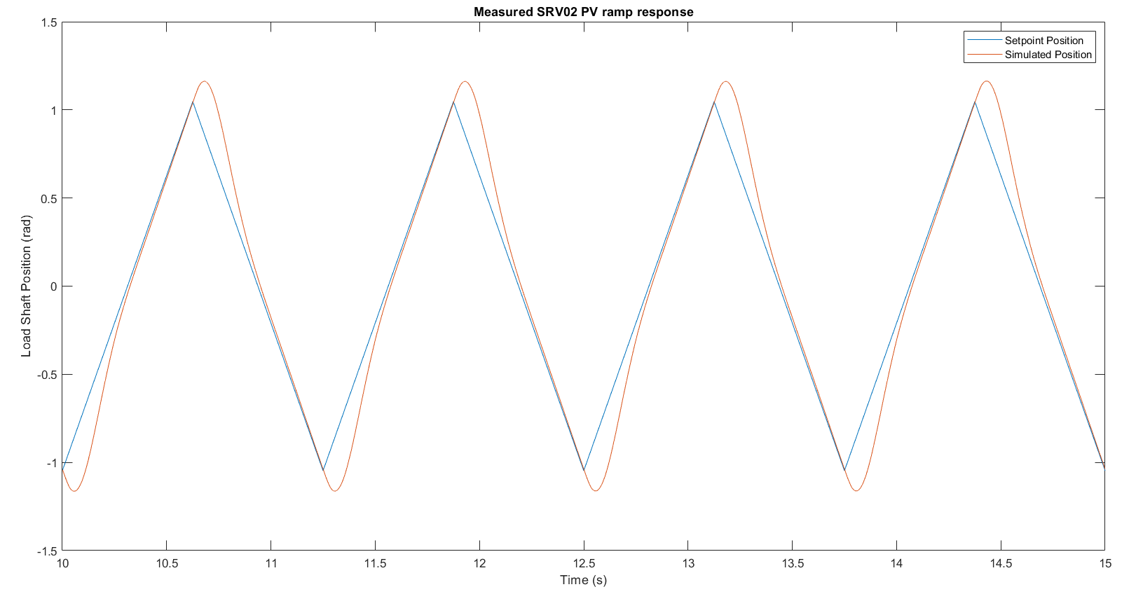
Ramp impl (PIV)	—	—	0.007

Hardware step response (PO = 7.86%) slightly exceeded the 5% design spec, attributable to friction and encoder quantization noise not captured in the model.
PIV reduced ramp e_ss from ~0.19 rad to ~0.007 rad — a 97% reduction by adding one integral term, directly validating the Type-2 behavior theory predicts.

PIV controller — measured ramp response on hardware, ess=0.007 rad (97% reduction vs PV) — Figure 7: PIV controller — hardware ramp response, e_ss=0.007 rad (97% reduction vs PV)

Valuable Takeaways

Transient specifications translate directly into controller gains. Mapping peak time and overshoot to ζ and ω_n, then to k_p and k_v, is a reusable workflow for any second-order position control problem, from aircraft actuators to CNC machine tool axes.
The type number of a control system determines what inputs it can track without error. PV (Type 1) tracks step positions but accumulates ramp error; PIV (Type 2) tracks both — this distinction drives integrator inclusion decisions in autopilot and flight controller design.
Hardware always differs from simulation. The 7.86% vs 5% overshoot discrepancy came from real-world nonlinearities. Recognizing and explaining this gap — rather than ignoring it — is what separates competent control engineers from those who only work in simulation.
Developed proficiency in the complete MATLAB/Simulink hardware-in-the-loop workflow, from analytical gain design and simulation validation through hardware implementation and performance characterization.